Projecting JunoCam images

Raw JunoCam images consist of several framelets, each corresponding to a different filter. As the spacecraft moves, the framelets correspond to different parts of the sky. To project the raw image to a map, we need to calculate the positions of each pixel in the image.

Also be sure to compile the C script in the projection/ folder. To do this, open the projection/ folder in a terminal, and run make.

Once those are done, import the projector functions. The first command points to the location of the JunoCamProjection module.

from junocam_projection.projector import Projector, create_image_from_grid
import cartopy.crs as ccrs
import numpy as np
import matplotlib.pyplot as plt

%matplotlib inline

The projection functions make use of the SPICE toolkit which read in kernel files that are produced by NAIF. These kernel files define the position of planets and spacecraft and are updated periodically.

To project JunoCam data, we will need the Juno kernels. These will be automatically downloaded from the NAIF website as needed. You will need to point to a location on your machine for where these files should be stored. You can store them in the same directory as your script, but if you expect that you will run this script in different directories, you should point to a central location. This will create a kernels/ folder and populate it with different kernels that define the Juno spacecraft and Jupiter coordinate systems. In the next cell, set KERNEL_DATAFOLDER to point to the kernels folder that was created.

WARNING: The downloaded data is on the order of several GBs for multiple PJs. Make sure you have the disk space for it

KERNEL_DATAFOLDER = "./kernels"

Now initialize the Projector class with the location of our image and metadata that’s associated with it. JunoCam images can be downloaded from the JunoCam Processing website. To process the raw images, be sure to select the JUNOCAM filter so as to filter out user generated images.

Click on the image, and download the images and metadata zips to this folder. Unzip them to produce theImageSet/ and DataSet/ folders. Note the name of metadata file inside the Dataset/ folder.

We initialize the Projector class by inputting the folder containing the images (ImageSet/), the metadata file (DataSet/xxxx-Metadata.json) and the location of the kernels. This example shows the included GRS image from Perijove 27 (ID: 8724). The code automatically determines the best value for the jitter in the image start time by fitting the limb of the planet (see timing note here).

proj = Projector("ImageSet/", "DataSet/8724-Metadata.json", KERNEL_DATAFOLDER)

Loading data for JNCE_2020154_27C00047_V01
Fetching kernels from NAIF server
Downloading ./kernels/spk/de442s.bsp

Downloading spk/de442s.bsp:   0%|                                                           | 0.00/31.2M [00:00<?, ?B/s]
Downloading spk/de442s.bsp:   6%|##8                                               | 1.80M/31.2M [00:00<00:01, 18.9MB/s]
Downloading spk/de442s.bsp:  18%|########7                                         | 5.49M/31.2M [00:00<00:00, 30.2MB/s]
Downloading spk/de442s.bsp:  27%|#############4                                    | 8.36M/31.2M [00:00<00:00, 26.0MB/s]
Downloading spk/de442s.bsp:  35%|#################4                                | 10.9M/31.2M [00:00<00:00, 24.9MB/s]
Downloading spk/de442s.bsp:  43%|#####################3                            | 13.3M/31.2M [00:00<00:00, 24.4MB/s]
Downloading spk/de442s.bsp:  50%|#########################                         | 15.7M/31.2M [00:00<00:00, 24.3MB/s]
Downloading spk/de442s.bsp:  58%|############################8                     | 18.0M/31.2M [00:00<00:00, 24.3MB/s]
Downloading spk/de442s.bsp:  66%|################################7                 | 20.5M/31.2M [00:00<00:00, 24.7MB/s]
Downloading spk/de442s.bsp:  73%|####################################5             | 22.8M/31.2M [00:00<00:00, 23.2MB/s]
Downloading spk/de442s.bsp:  80%|########################################1         | 25.0M/31.2M [00:01<00:00, 21.2MB/s]
Downloading spk/de442s.bsp:  87%|###########################################4      | 27.1M/31.2M [00:01<00:00, 20.9MB/s]
Downloading spk/de442s.bsp:  93%|##############################################6   | 29.1M/31.2M [00:01<00:00, 20.5MB/s]
7984it [00:01, 5573.16it/s] 100%|#################################################8| 31.1M/31.2M [00:01<00:00, 20.6MB/s]
Downloading spk/de442s.bsp: 100%|##################################################| 31.2M/31.2M [00:01<00:00, 22.7MB/s]

Downloading ./kernels/sclk/JNO_SCLKSCET.00187.tsc

Downloading sclk/JNO_SCLKSCET.00187.tsc:   0%|                                              | 0.00/35.7k [00:00<?, ?B/s]
9it [00:00, 9749.16it/s]
Downloading sclk/JNO_SCLKSCET.00187.tsc: 100%|#####################################| 35.7k/35.7k [00:00<00:00, 2.71MB/s]

Found 26 RGB frames

Decompanding: 100%|█████████████████████████████████████████████████████████████████████| 26/26 [00:05<00:00,  4.97it/s]
Finding jitter: 100%|█████████████████████████████████████████████████████████████████| 240/240 [01:34<00:00,  2.53it/s]

Found best jitter value of -28.0 ms

Once the object is initialized, we can project it. Call the process method, which can run in parallel with the num_procs argument. This call calculates the lat/lon of the center of each pixel in the original JunoCam framelet, correcting for barrel distortions (see Optical Distortions section here) and for interframe delay. This will project the image onto a HEALPix whose resolution can be controlled using the nside parameter and return the HEALPix 3-channel map array.

Note: This will take a couple minutes. Be sure to change the number of processors as needed.

proj.process(num_procs=10, apply_correction="none")

Projecting JNCE_2020154_27C00047_V01

Projecting framelets: 100%|█████████████████████████████████████████████████████████████| 78/78 [02:53<00:00,  2.22s/it]

Applying no correction

Under the hood, the algorithm first projects the data onto a frame at the mid-point of Juno’s trajectory for this image first before building the HEALPix map. The code will also generate a proj.framedata object which will contain information from individual framelets in the initial (moving) coordinate system. These correspond to the following data:

• proj.framedata.coords: The pixel coordinates in the mid-point frame

• proj.framedata.image and proj.framedata.rawimg: The flux (and Lommel-Seeliger correction) corrected and raw, decompanded image pixel values

• proj.framedata.lat and proj.framedata.lon: The latitude/longitude (SIII planetographic) of each pixel

• proj.framedata.emission and proj.framedata.incidence: The emission and incidence angles for each pixel (radians)

• proj.framedata.fluxcal: An initial calibration to remove viewing geometry effects

We can save the projected data to a NetCDF file so we can use it later without having to run this process again.

proj.save(proj.fname + ".nc")

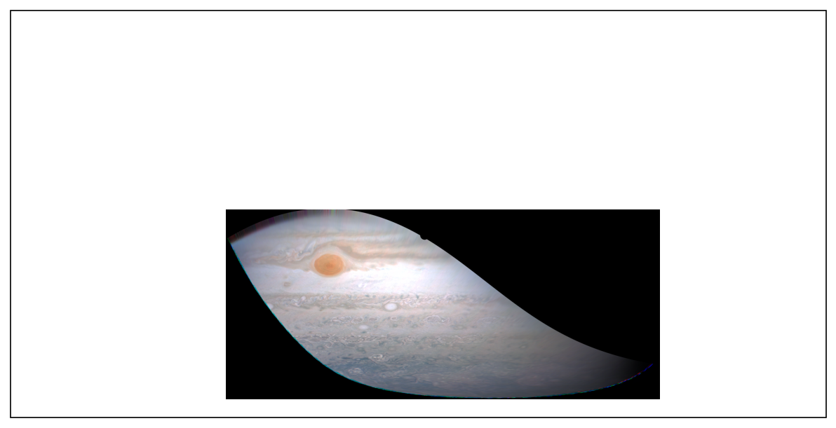
Then, let’s project it to a cylindrical projection and see how it looks! The resolution keyword is the pixel resolution in km/pixel.

m = proj.project_to_cylindrical(resolution=50)

Calculating image values at new locations

Building image: 100%|██████████████████████████████████████████████████████████████| 5925639/5925639 [00:13<00:00, 423277.75it/s]

globe = ccrs.Globe(ellipse=None, semimajor_axis=71492e3, semiminor_axis=66854e3)
platecarree = ccrs.PlateCarree(globe=globe)
fig, ax = plt.subplots(
    1, 1, figsize=(10, 8), dpi=150, subplot_kw={"projection": platecarree}
)
ax.imshow(
    m.image / np.percentile(m.image, 99),
    extent=(m.lon.min(), m.lon.max(), m.lat.min(), m.lat.max()),
    origin="lower",
)
ax.set_extent([-180, 180, -90, 90], crs=platecarree)
plt.show()

Clipping input data to the valid range for imshow with RGB data ([0..1] for floats or [0..255] for integers). Got range [0.0..5.996501961633278].

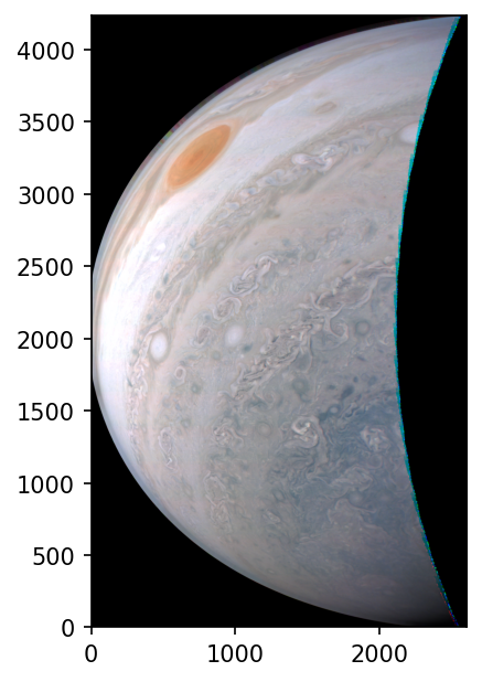
We can also see what the mid-point frame looks like by projecting directly onto the pixel coordinates returned by the projection

coords_new = np.transpose(proj.framedata.coords, (1, 0, 2, 3, 4)).reshape(3, -1, 2)
imgvals_new = np.transpose(proj.framedata.image, (1, 0, 2, 3)).reshape(3, -1)

# get the image extents in pixel coordinate space
x0 = np.nanmin(coords_new[:, :, 0])
x1 = np.nanmax(coords_new[:, :, 0])
y0 = np.nanmin(coords_new[:, :, 1])
y1 = np.nanmax(coords_new[:, :, 1])

# create the new frame which spans from the minimum to the maximum in (x, y)
x = np.arange(x0, x1, 0.5)
y = np.arange(y0, y1, 0.5)
X, Y = np.meshgrid(x, y)

# stack these coordinates together and create an indexer to loop through them
pix = np.column_stack([X.flatten(), Y.flatten()])
inds = np.asarray(range(len(pix)))

IMG = create_image_from_grid(
    coords_new, imgvals_new, inds, pix, X.shape, n_neighbor=10, max_dist=15
)

Calculating image values at new locations

Building image: 100%|████████████████████████████████████████████████████████████| 11018800/11018800 [01:44<00:00, 105113.79it/s]

plt.figure(dpi=150)
plt.imshow(IMG / np.percentile(IMG, 99), origin="lower")
plt.show()

Clipping input data to the valid range for imshow with RGB data ([0..1] for floats or [0..255] for integers). Got range [0.0..6.18392866670756].